Transformers: Origins
An unofficial origin story of the transformer neural network architecture.
This post tells the story of the transformer as a series of small discoveries starting from the first attempts at neural language modeling through to the invention of the transformer itself. The transformer did not come out of nowhere. As with anything in science, it is the culmination of a body of knowledge that builds on itself.
I do not know the authors of the first paper on the transformer (Vaswani et al. (2017) All You Need is Attention https://arxiv.org/abs/1706.03762). I do not know how they came up with this particular model architecture nor why all the details are what they are. However, the concepts that ultimately went into the transformer model architecture, like self-attention, can all be traced back to earlier incarnations of neural language models.
In this post, I walk through that chain of inventions from the basic recurrent neural network, through sequence-to-sequence networks with early versions of attention, to the final transformer architecture. I teach this sequence of concepts in my Natural Language Processing class at Georgia Tech, albeit in a more expansive form.
Language Models
A model is a simplified approximation of a complex phenomenon. A language model is a simplified approximation of an underlying, unknown process that results in the creation of words in documents. We don’t purport to know how language is produced, but it appears in writing — text documents — and it appears to have information in the sense of information theory: there is pattern to it.
The term language model has been around since at least 1976 (Jelinek, Continuous Speech Recognition by Statistical Methods, Proceedings of the IEEE vol. 64). It is now understood to be the probability of a word given a sequence of predecessor words:

This reads as: the probability of the word at position n, given the occurrence of a sequence of words in positions 1 through n-1.
The simplest form of language model is the unigram model (one word), which is simply the probability of a word occurring anywhere in the document. This is not particularly useful for generation. A bigram model (two words) is the probability of a word given the presence of the word that immediate precedes it. The preceding word can be considered a hint; it changes the probability of the subsequent word. A bigram model might be used as an early form of autocomplete. A trigram model is the probability of a word given the two precedings words. In general: an n-gram is the probability of a word given the preceding n-1 words. As n gets bigger, the choice of a word gets more informed by the presence of a bigger hint.
However, the size of n has an implication on the size of the model in terms of raw storage. A unigram model can be expressed as a table with a probability value associated with each word in a vocabulary (all possible words). A bigram model can be expressed as an N x N sized table where N is the number of possible words in the vocabulary. As we move to trigrams and 4-grams, the amount of information that needs to be stored becomes prohibitively large.
The concept of a language model does not imply how probabilities must be calculated. While we started by assuming precise calculations and probability tables, we can also consider approximation, wherein we are not guaranteed the precise probability, but one that is correct enough for practical purposes. One way of approximating an underlying language model is with deep neural networks, which can compress complex phenomenon in a set of learned parameters. A well-trained neural language model can express approximately the same relationship between words as a tabular language model.
Neural Language Models
In a perfect world, we would pump a bunch of words into a neural network and it would give us a value between 0 and 1 for each possible word that comes next.

Well, that just isn’t going to happen without figuring out a few things first. Neural networks operate on numerical inputs and outputs. So the first thing we need to do is figure out how to convert words into numbers.
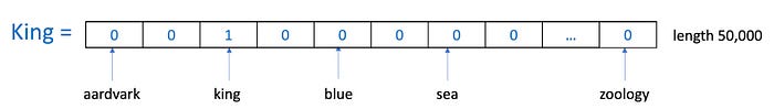
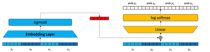
Each input word will be represented as a one-hot vector. A one-hot vector is an array the length of the vocabulary — the set of all words we wish our neural network to know. If we have a vocabulary of 50,000 words, then a one-hot vector is an array of length 50,000. This array is filled with zeros. Each position in the vector will correspond with a word in the vocabulary. Thus position 0 might correspond to “aardvark” and the 23rd position might represent “king”. We set exactly one position in the vector to 1.0 for the position we wish the one-hot vector to represent. Thus, the word “king” is also a one-hot vector with 22 zeros, a one, and 50,000–23 more zeros. Because each word is a one-hot vector with a specific position turned “on” (or “hot”), then we can also say the word “king” is also the token number 23.
The one-hot is useful because now we can build a neural network that takes a single word as input. This neural network will have 50,000 inputs. We just have to put a 1.0 in one of the inputs to tell the neural network which word we are giving it.
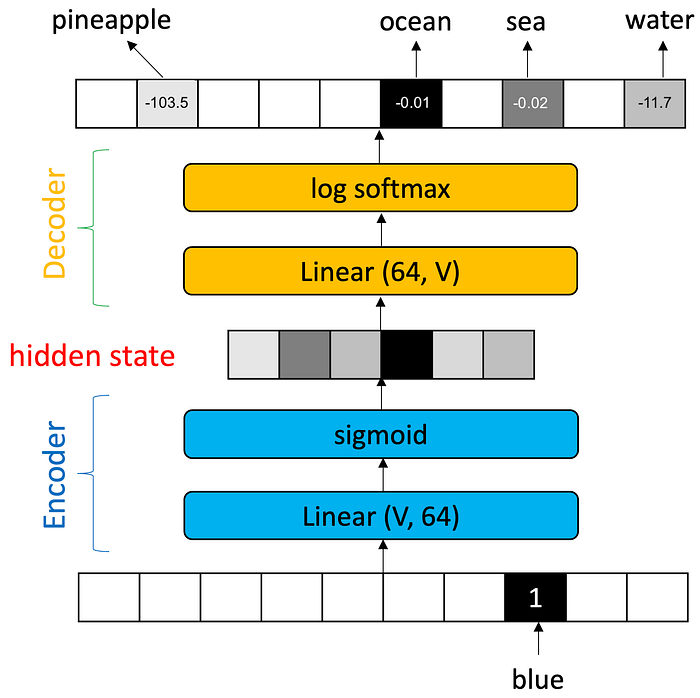
The output of the neural network can also have 50,000 outputs. However here we do not expect one output to have a 1.0 and the rest to have 0.0s. Instead, we will let the neural network provide any value for each output. These will be the “scores” for each word in the vocabulary and we can assume that the output with the highest score will be the word that is being chosen. Or we feed the vector of 50,000 scores into a softmax, which will normalize the output vector and we can treat it like a probability distribution.
(In reality, we will use a log_softmax(), which coverts numbers between 0 and 1 to a log scale so that 0 is negative infinity and 1 is 0. This means that the most probable word has a value close to zero and lower probability words have very small negative values. This helps us avoid floating point precision issues when probabilities get close to zero because the probabilities close to zero spread themselves out in log scale.)
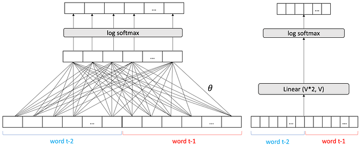
Here is what it looks like with one word coming in and one word coming out. On the left is a diagram in which I show the fully-connected layers so you can see all the parameters. On the right, I show the same network but as a computation graph.

The computation graph is simplified to avoid clutter; lines now just means everything produced from one layer (or module) is sent as inputs to the next layer (or module). This is called a computation graph.
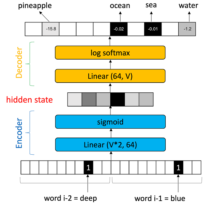
Now if we want a neural network with two words as input and produces a third word as output, we can build it with 100,000 inputs. The first 50,000 inputs will be a one-hot for the first word. The second 50,000 inputs will be a one-hot for the second word. It would look like this:
We are going to run into an issue where neural networks are going have to get really big if we want to be able to pump more words in. Plus, we might not know how long a sequence is going to be, so we don’t know how many inputs the neural network should have.
We will have to solve these issues, but let’s look a bit closer at what the inside of the neural network should look like.
Encoders and Decoders
In this section we introduce the concept of encoders and decoders.
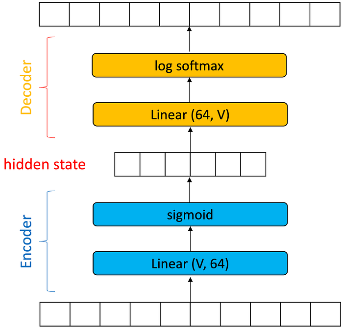
The easiest way to think about this is to think about two neural networks stacked one on top of the other. The bottom neural network’s job is to convert a word into some arbitrary, intermediate representation called a hidden state. The hidden state is just a vector of values that is much smaller than 50,000. We will call this network the encoder because it encodes the word. Think of it as a compression algorithm. It must compress 50,000 pieces of information into a smaller form, say 256 values.
The second neural network’s job is to take this hidden state and expand it out to 50,000. We call this network the decoder because it decodes the hidden state. Think of it as a decompression algorithm.
A good encoder-decoder network will have a “good” set of parameters for the linear layer in the encoder and a good set of parameters for the linear layer in the decoder. What is a “good” set of parameters? If the encoder parameters can compress the input into something that can be decompressed into a useful output, then the encoder-decoder network has been well-trained. If the hidden state is random then the decoder will also produce random scores.
As an illustrative example, consider an encoder-decoder network that computes the identity function. That is, given an input, the network produces an output identical to the input. This is just a toy problem, but it helps us understand how an encoder-decoder network is trained.
To train an encoder-decoder network to approximate the identity function, we give it a word, like “king”. We look at the output values. If the network tells us the most probable word is something other than “king”, then we know that either our encoder is wrong or our decoder is wrong or both.
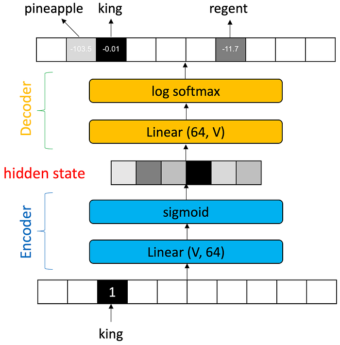
How far away the value in the “king” position is from 1.0 is the loss. The loss tells use how much the network needs to change. The backpropagation algorithm will tell us how much each parameter needs to change to reduce some of the loss. We do this for all words over and over again until we get the loss as close to zero as possible for all inputs.
Naturally we don’t usually want an identify function, we want something that predicts the next word. So instead of checking the output in the position that corresponds to the input word, we can grab a word from a training text document and check the output value in the position that corresponds to the next word in a training text. Now we have a bigram model:
And if we want a trigram, we can input two one-hots:
We are going to have to solve the problem of having arbitrary length inputs.
Recurrent Neural Networks
Texts are sequences. To process a sequence with a bigram model, we duplicate the network over and over again and put each word in the sequence in to see what comes out. Consider the problem of predicting that the next word in “the deep blue” should be “sea” and not “berry” if we just have bigram models.
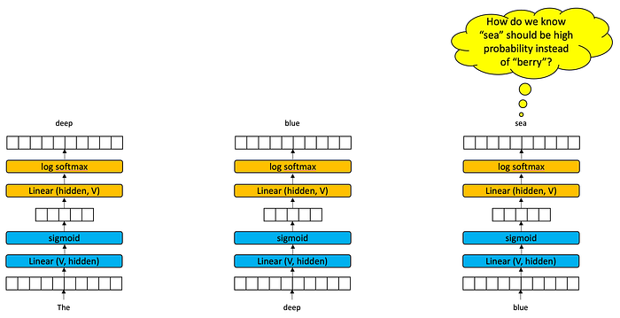
What reason do we have to believe that putting the word “blue” into an encoder-decoder should produce “sea” instead of “berry”. It may very well be that our training text has “blue berry” more often than “blue sea”. We don’t because each time slice — a word in a text — is processed independently of the prior words. What we need is a way for each time slice to pass information to its successor time slice.
Recall the hidden state. The reason we want an encoder-decoder is because the hidden state is a compressed representation of an input. We can’t look at the values in the hidden state and know what the input was, but those values were chosen by the neural network precisely because the decoder know what to do with it — it has information that is predictive of low-loss output. Also the hidden state is small relative to the inputs and outputs.
So what if we grabbed the hidden state out of the middle of a time slice and passed it to the next time slice. Now, instead of having an encoder-decoder with one input, we have an encoder-decoder with two inputs: the word at that time slice and the hidden vector from the previous time slice.
If the hidden state is meaningful, we should be able to learn a decoder that is responsive to both the current word and a hidden state. Moreover, the hidden state from time slice 2 will be a compression of the current word and the previous hidden state. And this new hidden state can be thought of as a “summary” of time slices 1 and 2. This will be pulled out and provided as an input to time slice 3. Now I think we can agree that the bigram model when we get to time slice 3 has a reasonable chance of being able to guess “sea” instead of “berry” because the hidden state might just encode some information about “the” and “deep”.
We call this a recurrent neural network (RNN). A recurrent neural network can theoretically process infinite-length texts by encoding each work in a text one time slice at a time and learning to pack useful information into the hidden state.
In practice: not so much.
Long Short-Term Memory Networks
The problem with vanilla RNNs is that they aren’t really very principled in how they pack concepts into the hidden state. This means two concepts can use the same values in the same vector positions. As the hidden state gets passed and each time slide builds a new hidden state, information can get lost or muddled up.
I’m going to gloss over Long Short-Term Memory (LSTM) models. The gist is that an LSTM model provides additional capability to preserve concepts that will probably be useful in the future and to forget concepts that are probably not going to be useful in the future. LSTMs have been shown to preserve context for longer sequences — it makes “short term memory” longer.
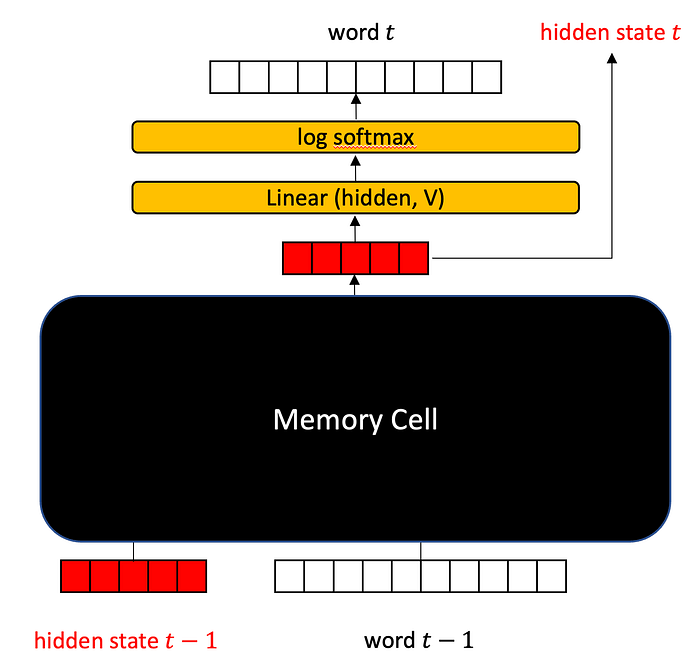
The LSTM passes not just a hidden state (red), but also a context state (green), which is information about what should be remembered and what should be forgotten. The word one-hot at a particular time slice is blue in the below diagram.
Anyway, all you need to know is that it works by passing both a hidden state and a context state between time slices, and you can just plop it into an RNN’s encoder.
Sequence-to-Sequence Networks
For certain types of generation problems, it is better to collect up a bunch of hidden states and generate everything all at once instead of generating time slice by time slice.
For example, in machine translation, we sometimes have to deal with swapping the order of words.

Also, the sequence lengths are not the same.
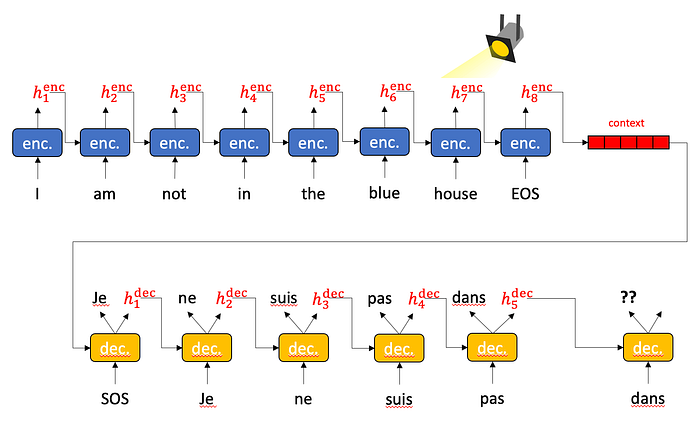
What I would like to do is to run everything in the source sequence through an RNN and build up a hidden state that captures the semantic meaning of the sequence. Then I would like to take this hidden state that represents the entire sentence and decode as many words as necessary to produce a faithful translation.
This is the genesis of the sequence-to-sequence model. It is the second most important model after the transformer, not because it is great, but because it introduces the concept of attention. But I’m getting ahead of myself.
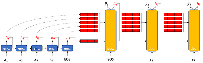
The seq2seq model runs every token in an input sequence through a copy of the encoder (which likely has an LSTM memory cell), passing the hidden state from time slice to time slice. However, we don’t decode. We’ve pulled the decoder off.

The hidden state we have at the end of the input sequence should hopefully represent the meaning of the entire sequence. Once we have that it is time to decode. But we do it a bit differently this time. We pass the input hidden state into the decoder. Since our decoder is not on top of the encoder, but beside it, we also pass in a token along with the hidden state. The decoder is thus a full encoder-decoder stack, encoding the input token alongside the hidden state.
(This side-by-side encoder-decoder scheme will be important, so remember it!)
What a weird thing to do. What tokens should the decoder get? The first time slide during decoding gets the start-of-sequence token, which is just a way of saying there is no incoming token information. This first time slice also gets the hidden state from the input sequence, which is hopefully chocked full of juicy information.
The decoder generates a token and an updated hidden. This output token is the real output. The hidden contains information about what was just produced. The generated token is the input token to the decoder at the next time slice, along side the new hidden. This continues until the decoder generates an end-of-sequence token.
The loss from each output token can be computed to train the fully-rolled out sequence-to-sequence model. A well-trained model should do a reasonable job of guessing tokens that match a target sequence, and it won’t be too bothered by reordering in machine translation because the hidden state will have already remembered that the verb needs to be negated and that nouns will be modified by adjectives.
One final small detail that will be important later. When the seq2seq model is early in training, it will produce a lot of garbage output tokens. One bad token feeds into the next time slice which will produce another garbage token, and so on. Training on garbage outputs is going to take a really long time to converge on anything. A way to speed this up is to do something called teacher forcing. Teacher forcing is just a weird term that means that instead of passing tokens from time slice to time slice during decoding, we force the next time slice to consume the target token for that time slice. We still compute the loss on the actual output, but we don’t let the next time slice see the garbage. That is, we correct the model after every mistake so it has good data to operate on. This seems like cheating. It is. You can only do this during training because at inference time you don’t have a target sequence. But it helps the model converge faster, and over time you can reduce the amount of teacher forcing.
Sequence Attention
The reason why seq2seq matters is three-fold. First, it introduces the notion of the side-by-side encoder and decoder as a reasonable thing to do. Second, it introduces teacher forcing as a reasonable thing to do. Third, seq2seq is amenable to sequence attention. These are all tools that will be really helpful when it is time to think about the transformer.
Let’s turn our attention to attention.
Seq2Seq, even with LSTM memory cells, can still muddle things up and forget things that are important for decoding. In some ways it is worse because we have to save up everything until the end of the input sentence and hope we saved all the right stuff. Perhaps decoder time slice 6 really only needs to know what was going on in the input at encoder time slice 7 because it needs to know the gender of the noun. Why should it have to deal with everything that got added to the hidden state after encoder time slice 7? Why should it have to deal with everything that got added to the hidden state during decoding prior to decoder time slice 6?
Sequence attention allows the decoder to reach back and pick out the most relevant hidden state from the encoding stage, pull it forward, and operate on it.
Sequence attention does exactly that. It collects up all the hidden states from all the encoder time slices and presents them to each decoder. But how to choose?
Behold the magic of a softmax followed by an inner product. Have you ever thought about softmax? I mean really thought about softmax? Softmax wants to be arg max. But you can’t really do an arg max in the middle of a neural network because arg max isn’t differentiable. Softmax wants one element in a vector — the biggest one — to become really close to 1.0 and all the rest to become really close to 0.0. In a perfect world, softmax would multiply all the hidden states by 0.0 except one, that is multiplied by 1.0 and thus survives. This then becomes the hidden state for the decoder. Sort of like this:
Well… that is what we want, but that isn’t quite what we get. Softmax doesn’t actually get one element to 1.0 and the rest to 0.0. Every element has a little bit of value, and sometimes several high-scoring elements have similar high values. We can treat the result of softmax as a probability distribution. We weight the hidden states by the probability and then add up the hidden states together. The highly probable hidden states keep most of their value while the low probability hidden states lose most of the value. When adding the hidden states together, the resulting hidden state is mostly the high probability components with a little bit of low probability sprinkled in. The result is a some composite of “house” and “in” and “not” and “I” and “am” and “the” to varying degrees.
Here is what the seq2seq decoder with sequence attention looks like inside.
The encoder just accumulates hidden states. The decoder does a lot of heavy lifting. This is because the decoder has to have an encoder inside it.
Here is a nicer, high-level picture of what the seq2seq with attention looks like:
The Transformer
Now it is finally time to turn to the Transformer.
The recurrent neural network is nice because it can have arbitrarily long input sequences. It means we don’t need to care about the input length. There was a point where we all agreed that we should not make really wide models. For example a simple feed forward network that read four tokens would require 4 x vocab_size inputs.

There was a time when most people would have said you were crazy to create a model like the one above. that this would be massively over-parameterized and really hard and expensive to train.
But what if you had an insane number of GPUs and an insane amount of training data and you didn’t care about how big your network was, how long it took to train, or how much it cost? You could make a really input window, say 1,024 tokens (or now we see transformers with 8,000 tokens, 32k tokens, or more), and pad any unused positions with zeros. This would open you up to some new architecture possibilities.
The Transformer pulls together three concepts:
- (1) Side-by-side encoder-decoder scheme. But this time the encoder and decoder will take in a sequence of many tokens all at once so we won’t need recurrence.
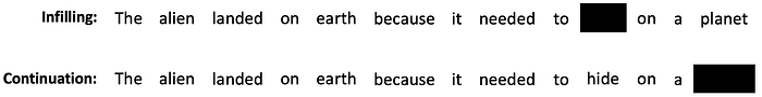
- (2) Masking. The input can be corrupted by masking out certain input and output positions so that the network must guess the missing tokens. By masking a word in the middle of a sequence, we can train a network to perform infilling. By masking the word at the end of a sequence, we can train a network to perform continuation (generation).
- (3) Self-attention. This is like sequence-attention from before, except instead of collecting up hidden states from previous time slices, all time steps are “flowing” through one gigantic feed-forward network. We are going to set up that network so that each time step can attend to every other time step. For one time step to attend to another time step means to pull a proportion of the representation from another encoded token in the sequence and add it to the encoding of the token at the attending time step.
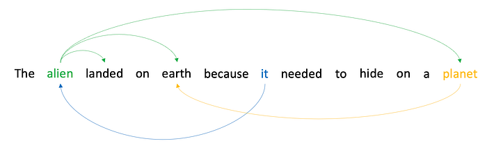
Self-attention is significant because it “transforms” the embedded representation of a token at one time step by incorporating some of the embedded representation from other, related tokens at other time steps. In the example above, the arrows denote relations between tokens that might be useful for decoding. For example, it would be really good to know that “it” also referred to “alien”. So if we needed to guess words relating to the alien, it would have some clues about how that concept has manifested before. Similarly, decoding is likely helped by knowing that “planet” and “earth” are the same thing. And even that “alien” is the thing that “landed”. It’s would be like having extra information packed into each word that takes all the guesswork out. Imagine reading the following:
The alien[pronoun:it; activity:landing, hiding, needing] landed[who:alien; where:earth] on earth[also:planet; context:where the alien lands] because it[who:alien] needed[who:alien,it; what:to hide] to hide[who:alien, it; where:earth, planet] on a planet[which:earth]
Pain in the butt for us, but literate adult humans are really good at figuring out context in sentences. An otherwise dumb computer is going to really appreciate all the extra information packed into each word.
And that is what self-attention does: it packs context into every embedded token at every time step.
So let’s look at how this works.
The Transformer Encoder, Part 1: The Embeddening
First of all, the transformer is still an encoder-decoder network. Here is the first part of the encoder:
In addition to a sequence of one-hots, a set of mask is also provided (the second token of four is masked).
The one-hots are embedded as normal.
But we want to know something about which token was in which time step position. We add a positional embedding to each token. The positional embedding is a small value that is added or subtracted to each element in each encoded token that is unique to each time step.
Next we make two copies of the result of the process so far. We call one the working copy and one the residual. The residual is the “official copy”. We are going to take that working copy and make a bunch of changes to it. Then we are going to take those modifications and add it back into the residual.
The changes we are going to make to the working copy are self-attention.
The Transformer Encoder, Part 2: Self-Attention
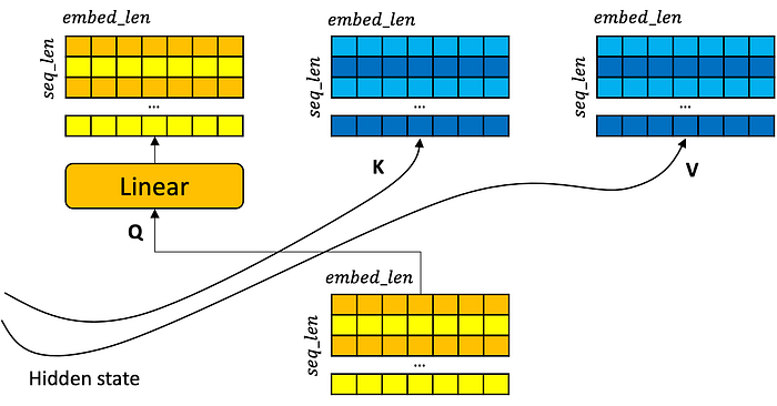
Self-attention starts with the working copy, which is a stack of token embeddings slightly adjusted with positional information.
We do some normalization, then we make three copies of this. We will call the copies Q, K, and V.
Before we go farther, I want you to think of a hash table. A hash table contains an ordered set of values. Each value is associated with a key. When you access a hash table you give a query. The query is matched to key. If there is an exact match to the key, then you get the associated value back.
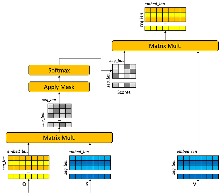
Self-attention is set up like a soft hash table. A bunch of queries are matched against a bunch of keys. We compute the similarity score for each pairing of queries and keys. The Q matrix is a stack of queries, one for each word. The K matrix is a stack of keys, one for each token. We compute the similarity score with… wait for it… an inner product of matrices and a softmax. Now you have pairwise scores between each token in the range of [0, 1].
How does the transformer know how similar things are? There is a linear layer applied to Q and K. The job of these linear layers are to transform Q and K, respectively, so that token embeddings are similar when the tokens are relevant to each other. The linear layers know this because if they transform the token embeddings properly, then the decoder will do a better job at guessing the masked token. If the linear layers don’t have the right parameters, they will make the embeddings effectively junk and the whole transformer gets no benefit.
Okay, so you learn some transformations to create a query Q and key K. And just so we are clear, Q and K are stacks of embedded tokens, one for each context position. Multiplying them together gives you an n x n matrix of scores where n is the context length. If any of those positions are masked, zero out the scores in that column. Run the n x n matrix through softmax so that your scores are between 0…1 and that each row sums to 1. We are going to call this matrix the attention scores. It tells us how much each position thinks every other positions is relevant. Because the linear layers should have made the embeddings of those positions similar.
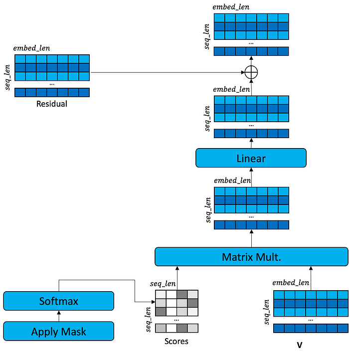
In a perfect world, softmax makes one element in an array 1.0 and all the rest 0.0. This doesn’t really happen, but suppose it does. It would look something like this: the 1s are selecting which row to grab from the V. Now the “retrieved” words from the V matrix are going forward instead of Q, and K.
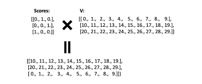
As before, softmax doesn’t give true 1s and 0s, so we get a bit of a blend of each embedded word, with the word in the most highly scored position being the most prominent component in the blend.
The take-away here, though, is that one word is being replaced by another word that is most “attended” to. there is some softness as to which word is retrieved, but it is not the original word going forward in each position.
The Transformer Encoder, Part 3: Return of the Residual
You might now be thinking: what happened to the input words in each position if they are all swapped out for different words drawn from V?
You might have noticed a residual being set aside earlier in the encoder. A residual is a pathway in the computation graph that bypasses the self-attention layers. In the transformer, the residual preserves the embedded input words and adds them back into the mix after self-attention. This allows the embedded input words to flow through the computation graph undisturbed by the self-attention process and get re-combined with the results of self-attention.
The Transformer Encoder, Part 4: Expansion and Collapse
Once the residual is merged back in, there is one more stage. A second residual is set aside (containing the original embedded input merged with the results of self-attention). Another round of layer normalization is performed. Then the words are expanded to a larger embedding size via linear layer, then collapsed to a smaller embedding size via linear layer. The second residual is then added back in.
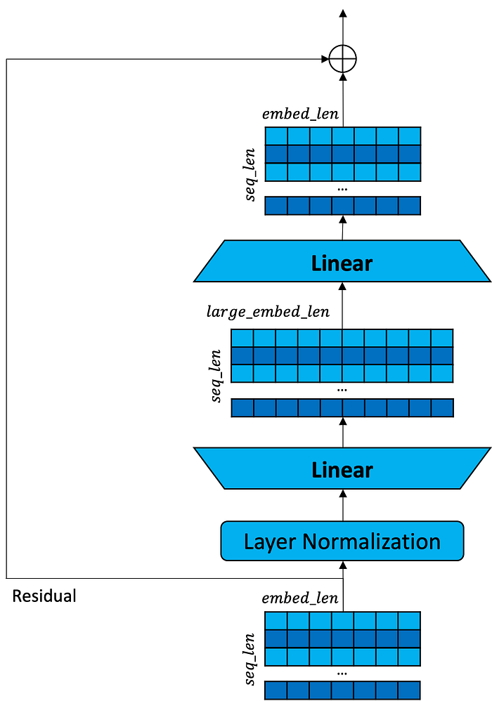
What does this expansion and collapse do? One interpretation is that expanding the embedding size allows room to shuffle things around. Many other neural architectures make layers bigger before making them smaller. This gives a neural network room to “be creative” and allocate positions to different abstract concepts. Collapsing the embedding size applies what is called a bottleneck. It forces the network to make compromises between concepts and map similar concepts to the same positions. Earlier encoder-decoder networks used bottleneck layers in the middle that were smaller than input and output layers to force the network to map similar words into the same compressed pattern. A second interpretation is that when multiple layers of self-attention are stacked on top of each other, it’s not practical to make embeddings progressively smaller as we go up the network, so one must make it bigger before making it smaller.
Regardless, the second residual is added back in after the fact, so these expansion-compression layers are useful or not, and if not, they don’t do any harm. When in doubt, use residuals and let the network figure out what is useful or not.
The Multi-Layer Transformer Encoder
This entire multi-stage encoder sequence is then repeated many times.
Interpreting the Transformer Encoder
We’ve been deep in the computation graph. Let’s take a step back and see if we understand the implications of all these transformations. Consider the following input sequence:
The kitten left its litter mates to use the litter [MASK]
When considering self-attention and the first residual, we can interpret the transformer encoder as transforming each input into a new word that represents a higher-level concept by merging an input word with another word in the sequence.
For example, “left” might attend to “kitten” creating a new word “kitten+left” that is essentially a special new verb for leaving that can only be done by kittens. Although I wrote “kitten+left”, it isn’t really making a new word like I just wrote. What is really happening inside the network is literally adding the embeddings of the original word, via the residual, and the attended word, making a new combination of embeddings that is neither the original word or the attended word.
This is very powerful. It is much easier to guess future words when there is no ambiguity about what a word means or how it is being used.
Likewise, the first “litter” might attend to “mates” creating “litter+mates” a new word that means the type of litter that is associated with mates. I am using the plus (+) symbol to indicate that the two words have been merged together in some way. This is not far from what is really happening because the residual — the encoding of the original word in a given position — is being added to the encoding of the word that was selected during the attention process (or more accurately, the weighted average of all the words according to similarity score). The second “litter” might attend to “use” creating a new concept “litter+use” that means the type of litter that can be used.
After one application of self-attention, we might think of the sequences as having been transformed into something like:
The+kitten kitten+left kitten+its litter+mates to kitten+use the litter+use [MASK]
Meaning the singular kitten did the leaving that only kittens can do from the litter of the kind that has mates belonging to it — the kitten — and going to the litter of the type that is used. As we go through subsequent rounds of self-attention, more complex concepts will be formed such as “kitten+litter+use” meaning the type of litter that can only be used by kittens. And so on.
What should go in the masked position? box? bin? mates? It is very likely that the network will learn that there is only one type of litter that is used exclusively by kittens and that is also referred to as a box. Once we have developed new words that subsume other words like this, there can be little ambiguity left when it comes to guessing the masked word.
The Transformer Decoder
Once the input sequence has been encoded, the decoder kicks in. Using the side-by-side encoder-decoder concept, the transformer decoder is a lot like the encoder. However, there is one important difference to self-attention: in the decoder, the Q matrix is an embedding of words produced by the decoder, but the K and V matrices come from the encoder.
Thus, the decoder is trying to learn to retrieve from the encoder. Very similar to how sequence attention worked in sequence-to-sequence models: a hidden state is passed from encoder to decoder to be combined with the decoder’s embedding of the input.
The rest is the same. Put a softmax on top of the decoder and unfold the embedded words and you have a probability distribution over the vocabulary for each sequence position. You only look at the masked position to compute the loss. Instead of cross-entropy, which only looks at the one spot in the vocabulary with the target token, to derive loss, the transformer uses KL divergence loss, which allows it to derive signal from all tokens in the vocabulary with respect to whether they should be 0s or 1s. This does the same thing as cross-entropy, but allows for more loss signal — not only do we look at whether we got close to the target token but we can also look at whether we should take loss for putting any non-zero score on tokens that are not targets. KL divergence loss is much more expensive to compute because it looks at the entire distribution instead of a single point in the distribution, but at this point we are not worried about computational cost.
Autoregression
Autoregression means inference on oneself. Transformers are autoregressive generators because they generate one word. That word gets added to the existing context and the next context, one word longer than before, is fed through the transformer again to create the second word. Then the new context, two words longer, is fed through the transformer. And so on.
This has some implications. If a word is generated, it gets added to the context no matter what. That means any word that gets generated gets “locked in” and the model then has the chance to have it attend to prior words and prior words to attend to the new word. That word affects the formation of new concepts and can drive the direction of the sequence generation henceforth. If a word is chosen that is locally optimal but not globally optimal, then future generation can take an unfortunate turn. Consider the following example: “Mark Riedl is a”. The model could continue this context with :
distinguished computer science professor at Georgia Tech who
Why “distinguished” because a lot of bios and profiles use that word, so it might just be a good default word to use here too. But the word “distinguished” could make the model then want to generate:
has won many awards including
because distinguished people win awards. But Mark Riedl hasn’t won many awards and so the model might not have learned anything that it can draw upon. So what can the model possibly generate next?
the Turing award in 2023.
The Turing award is an award given to distinguished computer scientists. The problem is that I have not won that award. I may not even be distinguished. But once the word “award” is chosen, then an award probably needs to be mentioned and some awards are more probable than others considering that “computer science” is now in the context.
We refer to this phenomenon wherein a word choice leads to successive choices that do not correlate with reality as hallucinations. The model cannot change its mind about the word “award” and must continue, introducing confabulations that may lead to more confabulations as concepts that are not true in the real world are successively added to the context.
Generalization vs Memorization
All recurrent neural networks and transformers are motivated by the intrinsic objective to reduce loss. There are two ways for a neural network to reduce loss: generalization and memorization.
Generalization stems from the identification of a general pattern that can be applied to new situations. For example, the model can learn that the word “drop” often precedes the word “fall”. The model doesn’t need to learn that “what happens when I drop a ball?” is different from “what happens when I drop a brick?” Generalization reduces error because it means the model is able to make a good guess about what word should come next. Generalization is an desirable property of all learning systems because it means complex phenomenon can be reduced to a relatively small number of parameters. Generalization, as a desirable property of a model, stems from the scientific principle of parsimony (also called Occam’s Razor), which states that when there are competing scientific theories, the simpler one should be preferred.
Memorization occurs in a neural network when it discovers that some number of parameters can be devoted to responding to a very specific input. For example, there is no general principle that can help a model respond to the input “What year was Alexander Hamilton born?” The model must either guess and receive loss, or it must devote some number of parameters to triggering the output layer to produce “1757” as the highest activating token. Memorization also reduces network loss because memorization means that it gets the next word prediction correct and therefore receives less loss. Thus, networks are incentivized to memorize as much as possible. However, the more parameters are used to memorize, the less capacity for generalization is available. Generalization isn’t just about responding to facts: generalization is also going to help with fluency, grammar, and so on.
Very large transformers have a lot of parameters, and as the number of parameters increases, there is a point where there is a diminishing return from generalization and no diminishing return from memorization. It is not a surprise that we see the largest language models being really good at question answering because a lot of unique pieces of information can be memorized. Whereas there used to be a scientific preference for small, parsimonious models, there is little incentive to measure parsimony when it comes to large language model being released as a product where real users are going to be using it to answer questions.
We can think a bit about the implications of self-attention for generalization and memorization. As we think about self-attention as assembling the clues about the response into higher-order concepts, memorization occurs when the model assembles higher order concepts that are unique and have a single possible response. “born+alexander+hamilton+year” will have an unique encoding that triggers one single possible answer. Similarly, for generalization, “happens+drop” will have an unique encoding that increases the probability of decoding the word “fall” (and “happens+drop+helium” will have a unique encoding that increases the probability of decoding the word “float”).
Prompting
The transformer, like the sequence-to-sequence models and other RNNs before it, are word continuation generators. They work best when the context is the beginning of a sequence and the expectation is that the rest of the sequence should be continued. Thus “Once upon a time” as a prompt will produce story-like continuations.
However, something interesting happens when models are bigger than 1 billion parameters. If we think of the context as the set of clues to what the user wants to see in the generated output, then large transformers are better at picking out clues from longer contexts. That means we can now do more than just provide the beginning of a sequence. The context can now include instructions for the output. For example we can give the model a context such as “Write a poem about Alexander Hamilton in the style of Eminem”. While this context is ostensibly the beginning of the a sequence to be continued, the attention mechanisms draw together elements from across the context and we get:
Yo, check it, I’m the man, Hamilton, ain’t no debate,
Born in the gutter, raised with a fiery fate,
A bastard child, no father, no name to claim,
But I carved my own path, carved my own lane.
This provides a new style of interacting with the model, and we now call the context a prompt. The bigger the model the more complicated the instructions in the the prompt can be.
There is nothing particularly special about a prompt. The attention mechanisms pick out words to merge. After many layers of attention, if the transformer has constructed the concept of “poem+style+eminem”, then the most reasonable next word after the prompt is going to be “Yo”. In this sense, the clues are the abstract concepts that are formed by repeated merges of residual and attended encodings to the point that ambiguity about which word should be generated is greatly reduced.
The transformer is very sensitive to the prompt because this kicks off the construction of concepts that will get used in generation going forward. The careful construction of the prompt can result in outputs that are closer or farther from what was intended. The manual search for a prompt that provides better results for an intended purpose is called prompt engineering.
In-Context Learning
Sometimes one wants outputs in a particular style or format. In-context learning is a process of prompting whereby examples of what the output should look like are given in the prompt. For example, if I want answers to questions to be written in subject-verb-object format, I might give some example questions and example answers. The attention mechanisms picks up on this pattern in the prompt and subsequent generation is more likely to match this pattern.
For example:
Provide answers to the following questions:
Q: What happened when Jack went up the hill?
A: Jack fell down
Q: What did the horsemen do when humpty fell down?
A: Horsemen reassembled humpty
Q: What did the wolf do to the grandmother?
A: Wolf ate grandmother
Then we concatenate the question we actually want answered:
Q: What did Hansel do when entering the witch’s house?
A:
The final “A:” gives it a clue that it should follow the established pattern.
In-context learning is a bit of a misnomer because learning typically refers to the updating of parameters in the neural network. In this case, the network has already learned how to use its linear encoder layers to convert input words into keys, queries, and values such that they attend to each other. No parameters are being changed. The neural network has already learned to use attention to mimic word patterns. However, it looks like the model is learning a pattern and then applying it.
Chain of Thought
Chain of Thought is a prompting strategy in which the prompt includes something along the lines of “think step by step”. This addition to the prompt does something interesting. There is a lot of context on the internet in which people break down concepts and explain things in a stepwise fashion. By adding this to a prompt, a large language model receives a clue about the desired pattern of the output, namely that there should be a lot of details laid out in a linear fashion. This turns out to improve the results of certain types of queries, especially pertaining to multi-step logic or mathematics.
Consider the example:
One of four people — two men (Jack and Mike) and two women (Carol and Lily) — was murdered. The following facts refer to the people mentioned:
(a) Jack’s sister argued exactly once with Carol’s legal husband after the murder.
(b) Mike’s sister argued twice with the victim’s legal spouse after the murder. Who was the victim?
This prompt might result in:
The victim is Jack.
which is wrong. the model is simply selecting one of the four names to be provided as the answer (actually the model is choosing a word from the vocabulary, and because attention is probably creating concepts like “murdered+jack” and “murdered+mike” and “murdered+carol” and “murdered+lily” then the four names “Jack”, “Mike”, “Carol”, and “Lily” are much probably selections than any other word). The model has a 25% chance of getting the answer right.
However, if one adds “think step by step” to the prompt, the output will be something more like:
If Jack and Lily are brother and sister then Mike and Carol are brother and sister. If this is the case then Jack and Lily cannot be spouses, and Mike and Carol cannot be spouses. Thus Jack must be married to Carol and Lily must be married to Mike. Thus Lily argued once with Jack and Carol argued twice with Lily, leaving Mike dead. Since there are no contradictions, the victim is Mike.”
As these words stream out of the model one by one and get added to the context, attention mechanisms build up more and more concepts like “Mike+Carol+brother+sister” and “Jack+Carol+married+spouse” and “Carol+Lily+argued+twice” so on. This greatly increases the probability of the word “Mike” being generated after “the victim is”.
In short, what is happening in Chain of Thought is that the “think step by step” part of the prompt causes the generation to elaborate with more details. These details are then attended to along with the original prompt, biasing the generation toward better answers.
Chain of Thought also helps with math. The challenge for math puzzles for LLMs is that many numbers are equally probable/improbable so when it comes time for the language model to autoregressively generate a number, there are many numbers that can be chosen with high probability. The LLM isn’t actually doing math, but probabilistically choosing numbers. However, chain of thought generation means that hard math problems that are rare in the original training corpus can be broken down into simpler math problems that the model might have seen during training and is thus more likely to probabilistically choose the right number.
Consider the following prompt:
At a restaurant, each adult meal costs $5 and kids eat free. If a group of 15 people came in and 8 were kids, how much would it cost for the group to eat?
Virtually any number could be chosen to be the continuation. However, with chain of thought prompting, the following might get generated:
To solve this problem, we need to determine how many adults there are in the group and how much they will pay for their meals.
Total number of people in the group: 15
Number of kids in the group: 8
Since the kids eat free, we can subtract the number of kids from the total group size to find the number of adults:
Number of adults=15−8=7
Each adult meal costs $5, so the total cost for the 7 adults is:
Total cost=7×5=35
Thus, the total cost for the group to eat is $35.
Consider what attention might be doing as it generates “number of adults=”. It is probably going to pull up existing numbers from the context, because that is what attention does. It is much more likely to pull 15 and 8 to get “15–8” and if it generates this, it has probably seen that simple math equation in its training data and know that “7” is a highly probably next choice. Similarly, now that “7” is in the context, then “7×5” is now probable. “7” was not in the original prompt, but it is available now to be attended to. And once again, the model has probably learned that 35 often succeeds “7×5” from its training data. No math has been done, but patterns have been applied.
Fine-Tuning
Fine-tuning is the concept of starting with a fully pre-trained model and providing a new, usually smaller, dataset to continue training on. Encountering new contexts and new continuations, the model will shift its weights to generate outputs more similar to the new data.
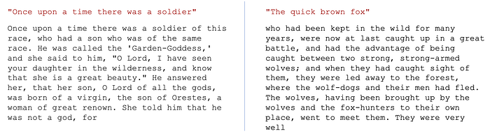
The following shows the pre-trained GPT-2 responses to two prompts:

If I were to take the text of J.R.R. Tolkien’s novel, The Silmarillion, and use it as additional training data, this new version of GPT-2 will start to adopt the style and topical preferences that are prevalent in the novel. The novel is of the fantasy genre, so the same prompts now produce different outputs:
Fine-tuning is a means of taking a general model and specializing it in a particular way.
Instruction Tuning
Consider the following scenarios:
- One prompts an LLM with “Write an essay about Alexander Hamilton” and it responds with “in twelve point font and is at least 5 pages long with references cited”.
- One prompts an LLM with a request for instructions on how to make poisonous gas, and the model responds with the instructions.
- One prompts an LLM with “write a poem about the big bang” and it fails to maintain any particular rhyme or meter.
The first scenario is about the model misunderstanding that the prompt is not the first line of a homework assignment instructions. The model has ostensibly trained on many sample exercises and is quite willing to generate the next part of the exercise. However, the user is probably wanting the model to respond to the prompt as if it were instructions instead of a prefix. In short, the model was not following instructions. The company or organization that makes or deploys the LLM would rather that the LLM is better at interpreting prompts as instructions instead of as prefixes to continue.
The second scenario is one in which the LLM does interpret the prompt correctly, but enables a dangerous activity. The company that deploys the LLM would rather the the LLM would refuse to answer.
The third scenario is one in which the LLM interprets the prompt correctly but presents a weakness, in this case maintaining a rhyme scheme and meter, and thus the result is not responsive to the prompt.
All of these scenarios are ones in which might be addressed by instruction tuning. Instruction tuning is a way of fine-tuning a pre-trained LLM to improve its responsiveness to prompts.
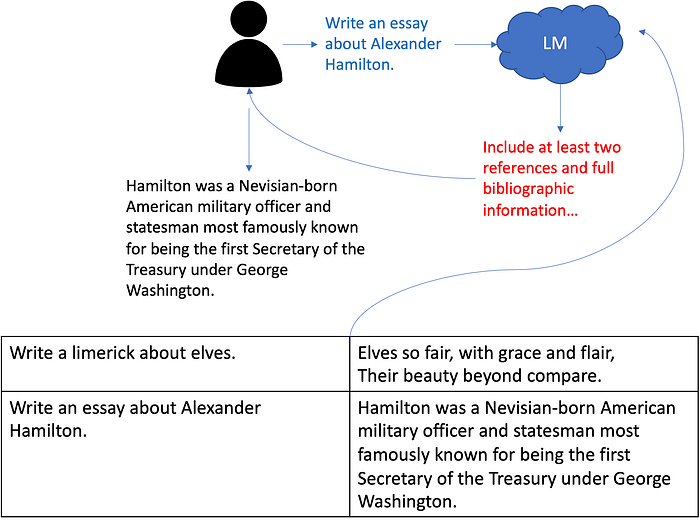
The most straight-forward way of instruction tuning is to:
- Human provides a prompt.
- Human receives a receives a response.
- Human rewrites the response to what a better response would have been.
- Create a dataset of prompts followed by human-authored responses.
- Fine-tune the model on the new data.
Thus if a prompt is “how do I make poison gas?”, the model might generate “first you buy bleach…”. The response is rewritten to be “I’m sorry, I cannot answer that.” The new data to train on is “how do I make poison gas? I’m sorry, I cannot answer that.” If fine-tuned properly, the model will either memorize that response or learn to generalize from certain prompts to certain new responses.
Reinforcement Learning with Human Feedback
Reinforcement Learning with Human Feedback (RLHF) is another way of instruction tuning. For the purposes of the discussion, reinforcement learning is just a way of using a non-differentiable score as loss during training. RLHF is just a fancy way of fine-tuning a language model. It happens in two stages.
The first stage is to train a classifier that can predict whether a human user will think an LLM response to a given prompt is appropriate or not.
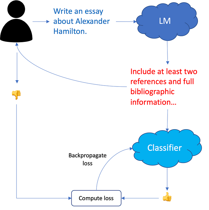
A prompt is given to an LLM, which provides a response. The user then rates the response. Another model, a classifier, attempts to predict the user’s rating. The user’s true rating is provided as a supervised training signal. This is done for many prompts and many responses until the classifier is able to accurately predict human feedback.
The second stage is to use the classifier to fine-tune the LLM. Fine-tuning has to happen a bit differently than before. Previously, we computed the loss of an LLM by looking at the input sequence and determining its output tokens match the response. Here we have a classifier that predicts how much a user will like the response. Fortunately, that rating can be turned into a loss (1.0 minus predicted rating because high score is equivalent to low loss, and vice versa) and that loss can be fed back into the LLM to adjust the weights like a regular loss. This is advantageous because, if the classifier can be trusted, then we can try many prompts, get many responses, classify them, and reward the LLM for good responses (low loss) and punish the LLM for bad responses (high loss).
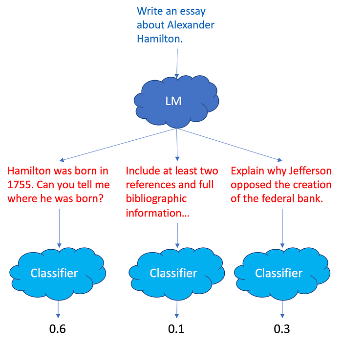
In particular, the LLM can produce multiple responses and the classifier can generate values that can be turned into loss to incentivize the LLM to respond in particular ways and avoid responding in other ways.
RLHF still needs a lot of training data, but this training data is used to train the classifier, and the classifier is used to fine-tune the LLM.